膨胀卷积与 1x1 卷积

在 [2017] Rethinking Atrous Convolution for Semantic Image Segmentation 中提到:

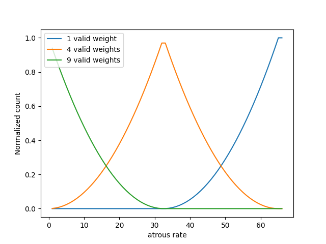
ASPP with different atrous rates effectively captures multi-scale information. However, we discover that as the sampling rate becomes larger, the number of valid filter weights (i.e., the weights that are applied to the valid feature region, instead of padded zeros) becomes smaller. In the extreme case where the rate value is close to the feature map size, the 3 × 3 filter, instead of capturing the whole image context, degenerates to a simple 1 × 1 filter since only the center filter weight is effective.

简言之, 膨胀卷积的 dilation rate (或称 sampling rate, atrous rate) 越大, 其越接近于 1x1 卷积的效果. 上面的文献还用 Fig. 4 展示了这一现象. 为了加深印象, 笔者写了如下代码来绘制与 Fig. 4 类似的图形.

import torch
import numpy as np
import matplotlib.pyplot as plt


if __name__ == '__main__':
    batch_size, num_channels, height, width = 1, 1, 65, 65
    x = torch.ones(batch_size, num_channels, height, width)

    weight = torch.ones(1, 1, 3, 3)
    num_valid_weights_1 = []
    num_valid_weights_4 = []
    num_valid_weights_9 = []
    dilations = range(1, height + 2)
    for dilation in dilations:
        y = torch.nn.functional.conv2d(x, weight, bias=None, stride=1, 
                                       padding=[dilation, dilation], 
                                       dilation=[dilation, dilation]) 
        num_valid_weights_1.append(len(torch.nonzero(y == 1)))
        num_valid_weights_4.append(len(torch.nonzero(y == 4)))
        num_valid_weights_9.append(len(torch.nonzero(y == 9)))
    num_valid_weights_1 = np.asarray(num_valid_weights_1) / np.prod(x.shape)
    num_valid_weights_4 = np.asarray(num_valid_weights_4) / np.prod(x.shape)
    num_valid_weights_9 = np.asarray(num_valid_weights_9) / np.prod(x.shape)
    plt.plot(dilations, num_valid_weights_1, label='1 valid weight')
    plt.plot(dilations, num_valid_weights_4, label='4 valid weights')
    plt.plot(dilations, num_valid_weights_9, label='9 valid weights')
    plt.xlabel('atrous rate')
    plt.ylabel('Normalized count')
    plt.legend(loc='best')
    plt.show()

输出为:

笔者还想到另外一种方式来展示这一现象, 如下代码:

import torch
import matplotlib.pyplot as plt


if __name__ == '__main__':
    batch_size, num_channels, height, width = 2, 8, 16, 16
    x = torch.randn(batch_size, num_channels, height, width)

    weight = torch.randn(4, 8, 3, 3)
    weight_1x1 = weight[:, :, 1:2, 1:2]
    y_1x1 = torch.nn.functional.conv2d(x, weight_1x1, bias=None, stride=1)
    dilations = range(1, height + 2)
    mae_list = []
    for dilation in range(1, height + 2):
        y = torch.nn.functional.conv2d(x, weight, bias=None, stride=1, 
                                       padding=[dilation, dilation], 
                                       dilation=[dilation, dilation]) 
        mae_list.append(torch.mean(torch.abs(y - y_1x1)))
    plt.plot(dilations, mae_list)
    plt.xlabel('atrous rate')
    plt.ylabel('mae')
    plt.legend(loc='best')
    plt.show()

输出为:

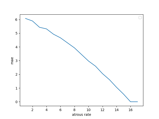
由上图可见, 膨胀卷积的结果与其对应 1x1 卷积的结果的 MAE 随着 dilation 的增大而减少, 当 dilation 大于等于 feature map 的尺寸时, 两者相等, 即膨胀卷积退化为 1x1 卷积.

更新记录

20210723, 发布

版权声明

保持署名-非商业用途-非衍生, 知识共享3.0协议.